
Computer Vision เป็นวิชาแขนงหนึ่งทางด้าน AI ( Artificial Intelligence ) ที่ว่าด้วยการทำให้ระบบสามารถประมวลผลภาพนิ่งหรือวีดิโอ เพื่อนำไปต่อยอดในด้านต่าง เช่น การวิเคราะห์ภาพ แยกแยะวัตถุในภาพ การติดตามวัตถุในวีดิโอเมื่อมีการเคลื่อนไหว และอื่นๆอีกมากมาย โดยมีเป้าหมายให้เทคนิคดังกล่าวนั้นแม่นยำและรวดเร็วเทียบเท่ากับมนุษย์
OpenCV จึงเป็น 1 ใน library tools ที่นิยมใช้ในการทำ Computer Visioning ด้วยภาษา python เพราะใช้งานง่ายและมีตัวอย่าง ( case study ) มากมายบนโลกอินเทอร์เน็ต
ด้วยความอยากรู้ผมจึงลองค้นหาในอินเทอร์เน็ตเกี่ยวกับ OpenCV ว่าจะลองเรียนอันไหนดีละบังเอิญว่าบนเว็บไซต์ OpenCV เขามีคอร์สฟรีให้เรียนด้วยแฮะก็เลยลองสมัครละก็ลงเรียนดู
โดยการที่จะได้ certificate จากทาง OpenCV university นั้นจะมี 2 ระดับก็คือ ระดับ honor (80%) กับ pass (60%) โดยวิธีการ grading จะเป็นการดูวีดิโอ และตอบ Quiz ในแต่ละ labs ให้ถูกต้อง
ระหว่างที่ผมนั่งเรียนอยู่ประมาณ 2-3 วัน มีเบอร์แปลกโทรมา เราก็นึกว่ามิจฉาชีพ แต่จริงๆแล้วเป็นเหมือนทีมงานของ OpenCV เขาโทรมาแนะแนวและแนะนำว่าเขามีคอร์สอื่นๆด้วยนะ ละก็แอบขายของเสียเงินนิดนึง รวมทั้งบอกว่าถ้าติดปัญหาอะไรสามารถ email มาได้เลย รู้สึกประทับใจมาก 555
มาพูดถึงเนื้อหาภายในคอร์สดีกว่าครับ นอกเรื่องซะเยอะเลย ตามที่กล่าวไปด้านบนเนื้อหาจะเป็นการ work along ด้วยการทำ lab ตามผู้สอนละมาตอบ Quiz โดยจะมี session ที่ถ้าเราสงสัยก็สามารถพิมพ์ถามทิ้งไว้ได้ เอาละได้เวลาอันสมควรแล้ว เรามาเข้าสู่เนื้อหากันดีกว่า ลุยกันน
Table of Content
- Course Introduction
- Getting Started with Images
- Basic Image Manipulation
- Image Annotation
- Image Enhancement
- Accessing the Camera
- Video Writing
- Image Filtering (Edge Detection)
- Image Feature and Alignment
- Panorama
- HDR
- Object Tracking
- Face Detection
- Tensorflow Object Detection
- Pose Estimation using OpenPose
Course Introduction
ในส่วนของพาร์ทแรกคอร์สจะแนะนำว่าต้องทำ quiz ได้เท่าไหร่ถึงจะได้ certificate และก็ให้ดูวีดิโอบทสัมภาษณ์คุณ Satya Mallick CEO ของ OpenCV.org และผมสรุปจากวีดิโอได้ดังนี้
- คุณควรที่จะเริ่มต้นจากพื้นฐานทางด้าน AI เสียก่อนที่จะกระโดดไปในหัวข้อที่มีรายละเอียดเชิงลึกที่ซับซ้อน
- PyTorch, OpenCV, Tensorflow and keras คือสิ่งที่เราควรรู้
- เมื่อเรียนรู้เกี่ยวกับ Deep Learning แล้วเราควรที่จะลองประยุกต์ใช้
- Developer ส่วนใหญ่มักโฟกัสไปที่ภาษา python เนื่องจากการใช้งานที่สะดวกในการเข้าถึงเนื้อหา Deep Learning ทั้งที่ภาษา C ก็สามารถทำได้เช่นกัน
- อย่าลืมที่จะติดตาม Trend ใหม่ๆเพื่ออัพเดทความรู้ของตัวเอง
Getting Started with Images
ปกติการใช้งาน OpenCV จะนิยมใช้กับ Numpy เพื่อให้มาจัดการ list of pixel ในภาพที่อ่านด้วย OpenCV ซึ่งก่อนที่เราจะไปทำจะสามารถนำไปประยุกต์ใช้ในงาน เช่น face recognition system, self driving car, หรือ งานด้าน medical เราควรที่จะทำความเข้าใจกับ ฟังก์ชั่นพื้นฐานเสียก่อน
1. How do we read image ?
ใน OpenCV นั้นเราสามารถอ่าน ไฟล์รูปภาพได้หลายนามสกุล ไม่ว่าจะเป็น JPG, PNG ,WEBP ทั้งยังสามารถเลือกตัวแปรเพื่อระบุว่าจะอ่านเป็นแบบโทนสีแบบใด เช่น สีเทา (grayscale) ภาพสี (colorful) หรือ โหลดภาพแบบเทียบเท่ากับที่ input เข้ามีค่า alpha สำหรับค่า opacity ก็ได้
cb_img = cv2.imread(filename, flag)flag สามารถ pass ค่า int หรือ constant variable ใน OpenCV ก็ได้
| Flag | Constant Variable | Description |
|---|---|---|
| -1 | cv2.IMREAD_UNCHANGED | Loads image as-is, including transparency (alpha channel) |
| 0 | cv2.IMREAD_GRAYSCALE | Loads image in grayscale (black & white) |
| 1 | cv2.IMREAD_COLOR | Loads a color image (BGR format) |
ใน OpenCV, ภาพที่โหลดด้วย cv2.imread() จะถูกเก็บเป็น NumPy array และใช้ BGR (Blue-Green-Red) แทนที่จะเป็น RGB (Red-Green-Blue) ซึ่งแตกต่างจากไลบรารีอื่นๆ เช่น Matplotlib หรือ PIL
2. Reading some attributes
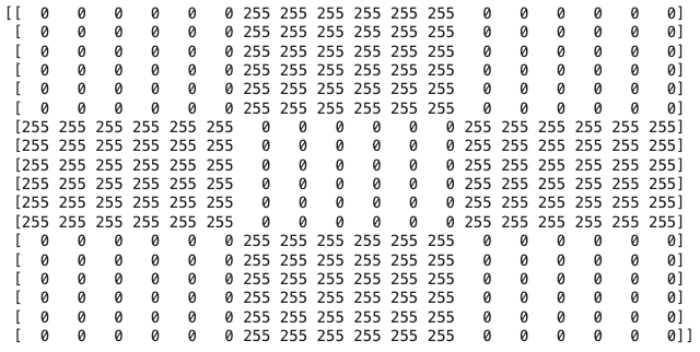
เราสามาถเรียก shape หรือ dtype เพื่อดู height & width กับ ประเภทข้อมูลได้จากค่าที่ return กลับมา
cb_img.shape ## (18,18)
cb_img.dtype ## uint8
3. Displaying Image with matplotlib
หากเราต้องการแสดงผลภาพที่อ่านจาก imread เราสามารถใช้ library matplotlib ในการอ่านค่า numpy array แต่บางครั้งหากเราอ่านภาพสีขาวดำเราจำเป็นที่จะต้องกำหนด parameter cmap เพื่อให้แสดงผลได้ถูกต้อง
plt.imshow(cb_img, cmap="gray")
4. Working with Color Images
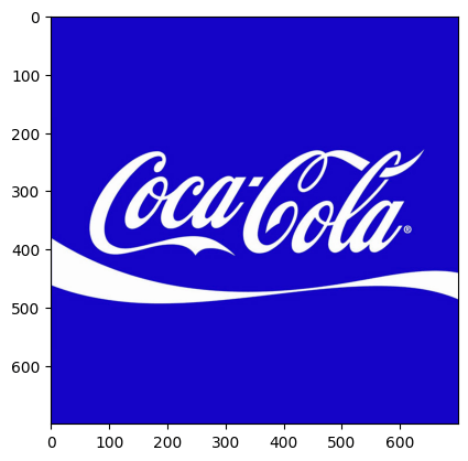
โดยปกติ หากเราพิมพ์ค่า attribute shape ของภาพขาวดำ (cv2.IMREAD_GRAYSCALE), ผลลัพธ์ที่ได้จะมีเพียง (height, width) เท่านั้น เนื่องจากภาพไม่มีช่องสี (color channel). แต่ถ้าเป็นภาพสี (cv2.IMREAD_COLOR), เราจะได้ค่า property ตัวที่ 3 นั้นก็คือ จำนวนช่องสี (Color Channels) ซึ่งใน OpenCV โดยปกติจะเป็น BGR (Blue, Green, Red)
print("Image size (H, W, C) is:", coke_img.shape) ## (700,700,3)ซึ่งถ้าเราเอาภาพสีที่อ่านด้วย imread ไปแสดงผลด้วย matplotlib จะทำให้สีภาพเปลี่ยนไปเนื่องจาก format BGR นั้นเอง เช่น

เพื่อให้ได้ค่าที่ถูกต้องเราต้องเอา NumPy array มาทำ array slicing ก่อน
coke_img_channels_reversed = coke_img[:, :, ::-1]เพียงเท่านี้เราก็จะได้ภาพสีที่ตรงกับ format ที่นิยมทั่วไป อย่าง RGB แล้ว
5. Splitting and Merging Color Channels
ในบางกรณีเรามีความจำเป็นต้องแยกสีของภาพ เพื่อประมวลผลที่ละช่อง ซึ่งการใช้ทั้ง BGR channel ดูจะเกินความจำเป็นไปหน่อย ด้วยเหตุนี้ OpenCV มีฟังก์ชัน cv2.split() เพื่อแยกช่องสีออกจากกัน และ cv2.merge() เพื่อรวมช่องสีกลับเข้าด้วยกัน
b, g, r = cv2.split(img) # แยกภาพออกเป็น B, G, R channelเราสามารถใช้ cv2.merge() เพื่อรวมช่องสี (Color Channels) กลับเป็นภาพเดิมได้ โดยส่งค่าช่องสีเป็น tuple เป็นอินพุต เช่น
img_merged = cv2.merge((r, g, b)) # รวมกลับเป็นภาพ แต่สลับเป็น RGBจากตรงนี้จะเห็นว่าเราสามารถเลือกวาง order ใหม่ได้ ก่อน merge เพื่อที่เราจะได้ไม่ต้องทำ array slicing
6. Converting Color Spaces
เราสามารถเรียกใช้งานฟังก์ชั่น cvtColor เพื่อแปลง Numpy Array นั้นไปอยู่ใน color channel ที่เราต้องการได้ เช่นจาก BGR → RGB หรือ BGR → Gray เป็นต้น สามารถดูตัวอย่างค่าคงที่ในตารางด้านล่าง
cv2.cvtColor(img_NZ_bgr, cv2.COLOR_BGR2HSV)ส่วนใหญ่แล้วก็จะมีค่าตัวแปรที่นิยมใช้ได้ดังนี้
| Code | Description |
cv2.COLOR_BGR2RGB | Converts BGR → RGB |
cv2.COLOR_RGB2BGR | Converts RGB → BGR |
cv2.COLOR_BGR2GRAY | Converts BGR → Grayscale |
cv2.COLOR_RGB2GRAY | Converts RGB → Grayscale |
cv2.COLOR_GRAY2BGR | Converts Grayscale → BGR |
cv2.COLOR_GRAY2RGB | Converts Grayscale → RGB |
cv2.COLOR_BGR2HSV | Converts BGR → HSV |
cv2.COLOR_RGB2HSV | Converts RGB → HSV |
cv2.COLOR_HSV2BGR | Converts HSV → BGR |
cv2.COLOR_HSV2RGB | Converts HSV → RGB |
7. Saving your modified image
หลังจากที่เราประมวลผลภาพแล้วเราสามารถ save Numpy Array กลับไปเป็นไฟล์ภาพได้ด้วย ฟังก์ชั่น cv2.imwrite()
cv2.imwrite("New_Zealand_Lake.png", img_NZ_bgr)Basic Image Manipulation
8. Changing Images Pixels
การที่เราอ่านไฟล์ภาพด้วย imread() และได้ค่าเป็น NumPy array นั้นแปลว่าเราสามารถแก้ไขภาพด้วยการเปลี่ยนค่าในแต่ละ index ได้ เช่น
cb_img[2,2] = 200 ## เปลี่ยนจาก 0-> 200
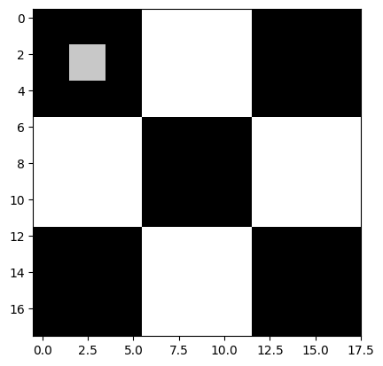
การเปลี่ยนค่าพิกเซลนี้สามารถใช้เพื่อการปรับแต่งภาพ เช่น การทำ Filter, Cropping, Masking หรือ Highlight พื้นที่บางจุด
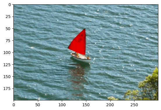
cropped_region = img_rgb[200:400, 300:600]
จากโค้ดด้านบน คือการเลือก แถว 200 – 399 กับ คอลัมน์ 300 – 599 หรือก็คือเอาภาพในช่วง (300,200) ถึง (599,300)นั้นเอง
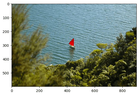
Caution ! ใน opencv กับ matplotlib จะให้ (0,0) อยู่มุมบนซ้ายของภาพ
9. Resizing Image
เราสามารถเรียกใช้คำสั่ง resize เพื่อปรับขนาดภาพ โดยอาศัย parameters ดังนี้
dst = resize(src,dsize[, dst[,fx[,fy[,interpolation]]]])| Parameter | Description |
|---|---|
src | ไฟล์ภาพต้นฉบับ (NumPy array) |
dsize | ขนาดของภาพที่ต้องการ (width, height) (ระบุขนาดใหม่โดยตรง) |
fx, fy | ตัวคูณขนาดภาพ (scale factor) ในแนวนอน (fx) และแนวตั้ง (fy) (ใช้เมื่อไม่กำหนด dsize) |
interpolation | วิธีการปรับขนาด เช่น cv2.INTER_LINEAR, cv2.INTER_CUBIC |
โดยการปรับขนาดภาพสามารถทำได้สองวิธี ดังนี้
✅ “หากต้องการกำหนดขนาดภาพแบบกำหนดเอง (เช่น 600×2000 พิกเซล)”
resized_image = cv2.resize(cropped_region, (600, 2000))✅ “หากต้องการปรับขนาดโดยใช้ Scale Factor (fx, fy) แทน dsize“
ในกรณีที่ใส่ dsize เป็น None เราสามาถใส่เป็น pass fx, fy ที่เป็น scale factor ในแนวนอนและแนวตั้ง ซึ่งหากค่า fx != fy จะทำให้ภาพ scale ผิดปกติได้
ตัวอย่างเช่น
resized_cropped_region_2x = cv2.resize(cropped_region, None, fx=1, fy=10)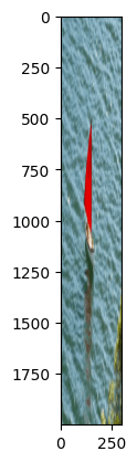
⚠ ข้อสังเกต:
- ถ้า
fx ≠ fyภาพอาจผิดสัดส่วน (ภาพบิดเบี้ยว) - ถ้า
dsizeถูกตั้งค่าเป็นNone, OpenCV จะใช้fxและfyแทน
10. Flipping Image
เราสามารถ หมุนภาพไปในทิศทางต่างๆ ได้ด้วยคำสั่ง flip()
dst = cv.flip(src, flipCode)| Parameter | Description |
|---|---|
src | ไฟล์ภาพต้นฉบับ (NumPy array) |
| flipCode | ค่าตัวเลขเพื่อระบุว่าจะ หมุนรอบแกนอะไร เช่น 0 สำหรับหมุนรอบแกน x ค่าบวก เช่น 1 หมุนรอบแกน y -1 สำหรับหมุนทั้งสองแกน |
Image Annotation
หลังจากที่เรารู้วิธีการจัดการกับรูปภาพแล้ว เรามาดูว่าถ้าหากเราอยากวาดหรือทำรอยบางอย่างบนภาพ รวมไปถึงการวางข้อความต้องทำอย่างไรกันน
11. Draw Line
เราสามารถเรียกใช้ method line() เพื่อเขียนเส้นบางอย่างบน ภาพที่เรา input ได้
img = cv2.line(img, pt1, pt2,color[, thickness[,lineType[, shift}}})| Parameter | Description |
|---|---|
| ไฟล์ภาพต้นฉบับ (NumPy array) |
| จุดเริ่มต้นของเส้น (x, y) |
| จุดสิ้นสุดของเส้น (x, y) |
| สีของเส้น (Tuple: |
| ความหนาของเส้น (ค่าเริ่มต้น = |
| lineType | ประเภทของเส้น ค่าเริ่มต้นคือ 8 สำหรับ 8-connected line |

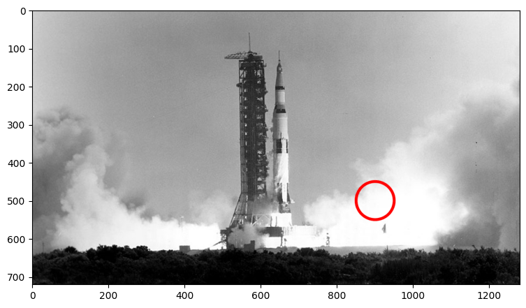
cv2.line(imageLine, (200,100), (400,100), (0,0,255), thickness = 5, lineType = cv2.LINE_AA)12. Draw a Circle
cv2.circle(imageCircle, c, r, (0,0,255), thicknesss=5, lineType=cv2.LINE_AA)| Parameter | Description |
|---|---|
img ไฟล์ภาพต้นฉบับ (NumPy array) | ไฟล์ภาพต้นฉบับ (NumPy array) |
c | |
r | รัศมี |
color | สีของเส้น (Tuple: (R, G, B)) |
thickness | ความหนาของเส้น (ค่าเริ่มต้น = 1 ไม่สามารถใช้ค่าลบได้) |
| lineType | ประเภทของเส้น ค่าเริ่มต้นคือ 8 สำหรับ 8-connected line |
parameter ก็คล้ายๆกับเส้นตรงเลยแต่จะเปลี่ยนเป็น จุดศูนย์กลางกับรัศมีแทน
13. Draw a Rectangle
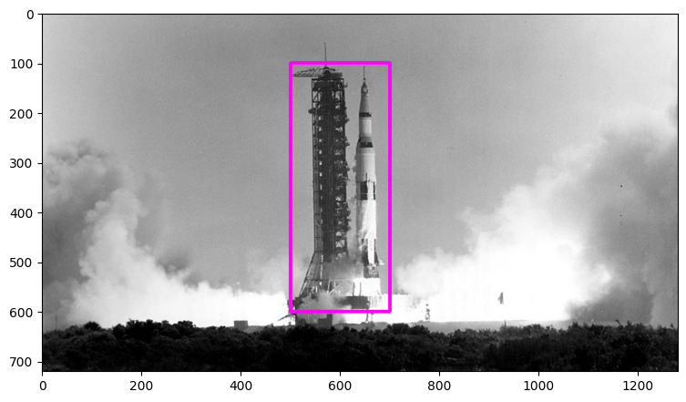
cv2.rectangle(imageRectangle, (500,100), (700,600), (255,0,255), thickness = 5, lineType=cv2.LINE_8)สำหรับการวาดเป็น รูป 4 เหลี่ยม ใช้ parameters เหมือนกับ line เลยแต่ต่างตรงที่ว่า จุดเริ่มกับจุดจบ จะใช้บอกว่าจะคลุมตั้งแต่จุดไหนถึงจุดไหน
14. Add Text in an Image
เราสามารถเพิ่มข้อความประกอบบนรูปภาพด้วยคำสั่ง putText()
cv2.putText(imageText, text,org, fontFace, fontScale, fontColor, fontThickness, cv2.LINE_AA)Here’s the formatted table for clarity and readability:
| Parameter | Description |
|---|---|
imageText | ไฟล์รูปภาพต้นฉบับ (NumPy array) |
text | ข้อความที่ต้องการใส่ในภาพ |
org | ตำแหน่งเริ่มต้นของข้อความ (x, y) |
fontFace | รูปแบบฟอนต์ (เช่น cv2.FONT_HERSHEY_PLAIN) |
fontScale | ขนาดของฟอนต์ |
fontColor | สีของฟอนต์ (Tuple: (R, G, B)) |
fontThickness | ความหนาของตัวหนังสือ |
lineType | ประเภทของเส้น |
Basic Image Enhancement
นอกจากการใช้งาน OpenCV ในด้าน Machine Learning และ Computer Vision แล้ว เรายังสามารถนำ OpenCV มาประยุกต์ใช้ในงานตกแต่งและปรับปรุงคุณภาพของภาพได้ เช่น การเพิ่ม ความสว่าง (Brightness), ความคมชัด (Contrast) หรือ การทำ Masking เพื่อไฮไลต์ส่วนที่สำคัญของภาพ
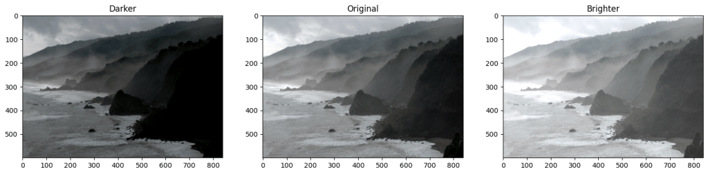
15. Adding Brightness
เราสามารถเรียกใช้ ฟังกชั่น add() หรือ substract() เพื่อปรับความ brightness ของภาพ ได้
matrix = np.ones(img_rgb.shape, dtype="uint8") * 50

img_rgb_brighter = cv2.add(img_rgb, matrix)
img_rgb_darker   = cv2.subtract(img_rgb, matrix)
จากตัวอย่าง เราสร้างเมทริกซ์ (matrix) โดยใช้ขนาดเดียวกับภาพต้นฉบับ และกำหนดประเภทข้อมูลเป็น uint8 จากนั้นนำเมทริกซ์นี้มาคูณด้วยค่าที่ต้องการ แล้วส่งผลลัพธ์เข้าไปในเมทอด เพื่อปรับความสว่างของภาพ
โดย add() และ substract จะรับ parameters สองตัวได้แก่ NumPy Array ที่เราจะใช้เป็นฐาน และ Numpy Array ที่จะเข้ามาปรับปรุง
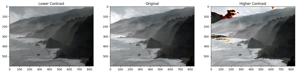
16. ปรับ Contrast ด้วย cv2.multiply()
เราสามารถปรับค่า Contrast ของภาพโดยใช้ cv2.multiply(), แต่ต้องระวังว่าเมื่อค่าพิกเซลที่คูณกันเกิน 255 อาจเกิด overflow ซึ่งทำให้สีของภาพเพี้ยนได้ ดังนั้น ควรใช้ numpy.clip() เพื่อลดค่าพิกเซลให้อยู่ในช่วง [0, 255]
matrix_low_contrast = np.ones(img_rgb.shape) * 0.8
matrix_high_contast = np.ones(img_rgb.shape) * 1.2

img_rgb_lower  = np.uint8(cv2.multiply(np.float64(img_rgb), matrix_low_contrast))
img_rgb_higher = np.uint8(np.clip(cv2.multiply(np.float64(img_rgb), matrix_high_contast), 0, 255))
การลด Contrast ใช้ตัวคูณ < 1 ส่วนการเพิ่ม Contrast ใช้ตัวคูณ > 1 และใช้ clip() เพื่อให้ค่าพิกเซลไม่เกินช่วงที่กำหนด

หรือเราสามารถเลือกใช้เป็น method threshold() ซึ่งจะเปลี่ยนค่าใน NumPy Array ให้เป็น 255 หากเกินค่าที่เรากำหนด และ 0 ในกรณีที่ต่ำกว่า
retval, img_thresh = cv2.threshold(img_read, 100, 255, cv2.THRESH_BINARY)หากค่าพิกเซลเกิน 100 ก็ให้ตั้งค่าเป็น 255 หรือสีขาว ถ้าน้อยกว่าก็เป็น 0 หรือ สีดำ ซึ่งเราสามารถกำหนดวิธีการตั้งค่าเมื่อเกิน THRESHOLD ผ่าน parameters ตัวสุดท้าายอย่าง type
| Thresholding Type | Description |
|---|---|
cv2.THRESH_BINARY | Pixels ≥ thresh → 255, else 0. |
cv2.THRESH_BINARY_INV | Inverse: Pixels ≥ thresh → 0, else 255. |
cv2.THRESH_TRUNC | Pixels ≥ thresh → set to thresh, else unchanged. |
cv2.THRESH_TOZERO | Pixels < thresh → set to 0, else unchanged. |
cv2.THRESH_TOZERO_INV | Pixels ≥ thresh → set to 0, else unchanged. |
Thresholding สามารถนำไปใช้กับการแยกภาพออกจากพื้นหลัง (Background Removal), OCR, X-ray และ MRI scan ได้ แต่ต้องใช้กับ ภาพ Grayscale เท่านั้น
ในบางกรณี การใช้ cv2.threshold() อาจไม่เพียงพอ เช่น ถ้าภาพมีแสงที่ไม่สม่ำเสมอ เราสามารถใช้ cv2.adaptiveThreshold() เพื่อให้ OpenCV คำนวณค่า Threshold ในแต่ละส่วนของภาพโดยอัตโนมัติ โดยภายใต้ฟังก์ชั่นดังกล่าวคือสูตรดังนี้
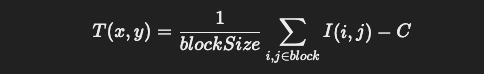
Adaptive Thresholding เหมาะสำหรับภาพที่มีแสงไม่สม่ำเสมอ เช่น เอกสารที่มีเงา หรือภาพ X-ray ที่ต้องการแยกโครงสร้างที่มีความเข้มแตกต่างกัน

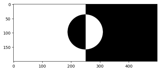
17. การทำ BITWISE AND OR XOR NOT
method ตระกูล bitwise-{and,or, xor, not} นั้นช่วยให้การ เอาภาพสองภาพมาซ้อนกันนั้นทำไปได้อย่างมีประสิทธิภาพ เช่นการ ทำ masking (การซ่อนหรือเลือกบางส่วนของภาพ) แต่การทำ bitwise นั้นเหมาะใช้กับภาพขาวดำ (Grayscale) หรือภาพที่เป็น Binary Mask (ค่าพิกเซลเป็น 0 หรือ 255 เท่านั้น)

Bitwise AND Operator
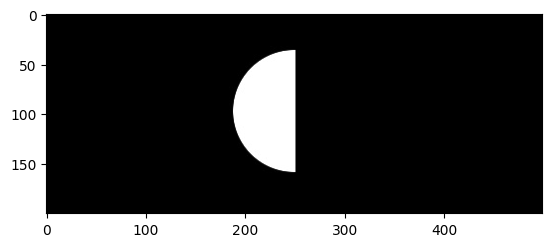
Bitwise OR Operator
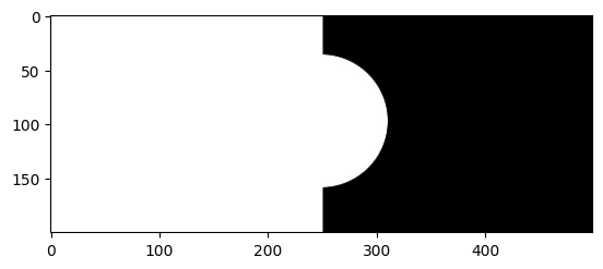
Bitwise XOR Operator
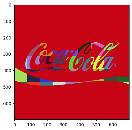
โดยใน แล๊ปจะพาดูการทำ Masking ของรูป brand Coca Cola กับภาพสี
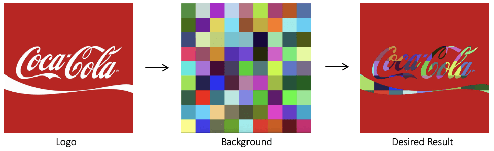
โดยในตอนแรกนั้น เราจะเริ่มจากการแปลงด้วย cvtColor เพื่อเปลี่ยนเป็น grayscale ก่อน
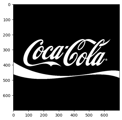
จากนั้นก็ใช้ ภาพด้านบนเป็น mask ให้กับภาพหลากสีที่เป็น background เราก็จะได้
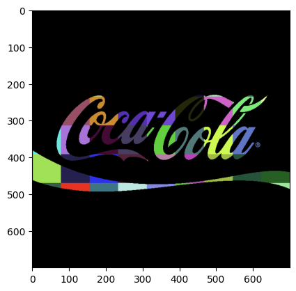
จากกนั้นให้ ให้ bitwise_not กลับ coca cola brand เพื่อให้สีขาวไปอยู่ด้านนอกตัวโลโก้ เพื่อที่เราจะเอามา ทำ masking
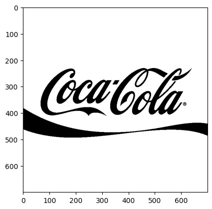
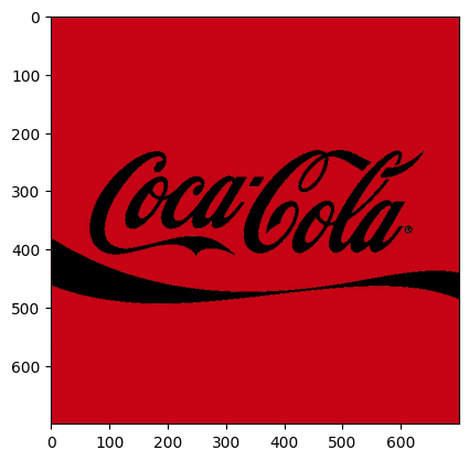
จากนั้นก็เอาภาพสองภาพมารวมกันโดย add() ก็จะได้ภาพสุดท้าย
img_bgr =cv2.imread("coca-cola-logo.png")

img_rgb = cv2.cvtColor(img_bgr, cv2.COLOR_BGR2RGB)
img_background_bgr = cv2.imread("checkerboard_color.png")
img_background_rgb = cv2.cvtColor(img_background_bgr, cv2.COLOR_BGR2RGB)

img_background_rgb = cv2.resize(img_background_rgb, (logo_w, logo_h), interpolation=cv2.INTER_AREA)
img_gray = cv2.cvtColor(img_rgb, cv2.COLOR_RGB2GRAY)
retval, img_mask = cv2.threshold(img_gray, 127, 255, cv2.THRESH_BINARY)
img_mask_inv = cv2.bitwise_not(img_mask)
img_background = cv2.bitwise_and(img_background_rgb, img_background_rgb, mask = img_mask)
img_foreground = cv2.bitwise_and(img_rgb, img_rgb, mask = img_mask_inv)
result = cv2.add(img_background, img_foreground)
Accessing the Camera
เนื้อหา แล๊ปที่ผ่านมาจะเกี่ยวกับรูปภาพซะส่วนใหญ่ ในแล๊ปถัดๆไปของทาง OpenCV จะเริ่มมีการสอนเกี่ยวกับการใช้ วีดิโอด้วยการสอนการเปิดใช้งานกล้องผ่านทาง OpenCV ก่อนจะพาไปดูว่าเราสามารถยุกต์อะไรได้บ้าง ไปดูกันเลยครับ
18. How to use your camera via opencv
น OpenCV เราสามารถใช้ cv2.VideoCapture() เพื่อเปิดกล้องและอ่านข้อมูลภาพแบบวิดีโอ ซึ่งสามารถนำไปประยุกต์ใช้ในงาน Object Tracking, Face Detection, หรือ Motion Detection ได้
import cv2
import sys


s = 0
if len(sys.argv) > 1:
    s = sys.argv[1]

source = cv2.VideoCapture(s)

win_name = 'Camera Preview'
cv2.namedWindow(win_name, cv2.WINDOW_NORMAL)

while cv2.waitKey(1) != 27:
    has_frame, frame = source.read()
    if not has_frame:
        break
    cv2.imshow(win_name, frame)

source.release()
cv2.destroyWindow(win_name)
Video Writing
การบันทึก (save) หรือดึงข้อมูลวิดีโอ (extract) เป็นสิ่งสำคัญในหลายงาน เช่น กล้องวงจรปิด (CCTV) ที่ต้องบันทึกช่วงเวลาสำคัญเพื่อใช้เป็นหลักฐาน หรือการประมวลผลวิดีโอในงานคอมพิวเตอร์วิทัศน์ เช่น Object Tracking หรือ Motion Detection
ปกติแล้วเราก็จะใช้ VideoCapture อ่านไฟล์ วีดิโอแต่ต้องระวังว่า frame ที่เรา read มานั้นจะให้ภาพใน color channel BGR เราต้องทำ slicing ก่อน
19 Writing Video using OpenCV
ใน OpenCV เราสามารถใช้ cv2.VideoWriter() เพื่อบันทึกวิดีโอที่ถูกอ่านหรือประมวลผล โดยต้องกำหนดชื่อไฟล์, รูปแบบการบีบอัด (codec), อัตราเฟรม (FPS) และขนาดเฟรมของวิดีโอ
VideoWriter object = cv.VideoWriter(filename, fourcc, fps, frameSize )
| Parameter | Description |
|---|---|
filename | ชื่อไฟล์output |
fourcc | 4-character code ที่ใช้ compress frames ซึ่งเราสามารถดูโค้ดได้บน เว็บไซต์ documentation ของทาง OpenCV ได้ |
fps | อัตราเฟรมต่อวินาที (Frames Per Second) ของวิดีโอที่สร้าง |
frameSize | ขนาดของเฟรมวิดีโอ (width, height) |
# Default resolutions of the frame are obtained.
# Convert the resolutions from float to integer.
frame_width = int(cap.get(3))
frame_height = int(cap.get(4))

# Define the codec and create VideoWriter object.
out_avi = cv2.VideoWriter("race_car_out.avi", cv2.VideoWriter_fourcc("M", "J", "P", "G"), 10, (frame_width, frame_height))

out_mp4 = cv2.VideoWriter("race_car_out.mp4", cv2.VideoWriter_fourcc(*"XVID"), 10, (frame_width, frame_height))
# Read until video is completed
while cap.isOpened():
    # Capture frame-by-frame
    ret, frame = cap.read()

    if ret:
        # Write the frame to the output files
        out_avi.write(frame)
        out_mp4.write(frame)

    # Break the loop
    else:
        break
# When everything done, release the VideoCapture and VideoWriter objects
cap.release()
out_avi.release()
out_mp4.release()
🔹 เปรียบเทียบ Codec ที่นิยมใช้
| Codec | File Format | Description |
|---|---|---|
"XVID" | .avi | ใช้กันอย่างแพร่หลาย, ขนาดไฟล์ไม่ใหญ่เกินไป |
"MP4V" | .mp4 | รองรับการใช้งานบนอุปกรณ์ทั่วไป |
"MJPG" | .avi | ใช้สำหรับการบันทึกภาพที่ไม่ต้องการบีบอัดมาก |
"H264" | .mp4 | บีบอัดได้ดี, ใช้พื้นที่น้อย |
Image Filtering ( Edging Detection )
20. Canny Edge Detection
Edge Detection เป็นเทคนิคที่ช่วยระบุ ขอบของวัตถุในภาพ โดยตรวจหาการเปลี่ยนแปลงของสีหรือความเข้มของพิกเซล ซึ่งสามารถใช้ในการระบุตำแหน่ง มุม (Corners) หรือ ขอบวัตถุ (Edges) ได้ง่ายขึ้น
ซึ่งการทำ Edge Detection มีหลายวิธี เช่น
| Method | Description |
|---|---|
Laplacian Operator | ใช้ Second–Order Derivative ตรวจจับขอบได้ไว แต่ไวต่อ Noise |
Sobel Operator | ใช้ First-Order Derivative คำนวณแนวขอบในแนวแกน X และ Y |
Canny Edge Detection | วิธีที่นิยมใช้มากที่สุด เพราะให้ผลลัพธ์ที่คมชัด แต่มีค่าใช้จ่ายสูงกว่าวิธีอื่น |
โดยใน โค้ดตัวอย่างนี้จะมีเรียกใช้ฟังก์ชั่น Canny() เพื่อให้ดูตัวอย่างภาพ และ วิธีการหา corners หรือ key features ในภาพ ด้วยวิธี Shi-Tomasi Corner Detection ( goodFeaturesToTrack() )
“การทำ Edge Detection จะมีประสิทธิภาพกับภาพแบบ Grayscale”
import cv2
import sys
import numpy

PREVIEW  = 0  # Preview Mode
BLUR     = 1  # Blurring Filter
FEATURES = 2  # Corner Feature Detector
CANNY    = 3  # Canny Edge Detector

feature_params = dict(maxCorners=500, qualityLevel=0.2, minDistance=15, blockSize=9)
s = 0
if len(sys.argv) > 1:
    s = sys.argv[1]

image_filter = PREVIEW
alive = True

win_name = "Camera Filters"
cv2.namedWindow(win_name, cv2.WINDOW_NORMAL)
result = None

source = cv2.VideoCapture(s)

while alive:
    has_frame, frame = source.read()
    if not has_frame:
        break

    frame = cv2.flip(frame, 1)

    if image_filter == PREVIEW:
        result = frame
    elif image_filter == CANNY:
        result = cv2.Canny(frame, 80, 150)
    elif image_filter == BLUR:
        result = cv2.blur(frame, (13, 13))
    elif image_filter == FEATURES:
        result = frame
        frame_gray = cv2.cvtColor(frame, cv2.COLOR_BGR2GRAY)
        corners = cv2.goodFeaturesToTrack(frame_gray, **feature_params)
        if corners is not None:
            for x, y in numpy.float32(corners).reshape(-1, 2):
                cv2.circle(result, (x, y), 10, (0, 255, 0), 1)

    cv2.imshow(win_name, result)

    key = cv2.waitKey(1)
    if key == ord("Q") or key == ord("q") or key == 27:
        alive = False
    elif key == ord("C") or key == ord("c"):
        image_filter = CANNY
    elif key == ord("B") or key == ord("b"):
        image_filter = BLUR
    elif key == ord("F") or key == ord("f"):
        image_filter = FEATURES
    elif key == ord("P") or key == ord("p"):
        image_filter = PREVIEW

source.release()
cv2.destroyWindow(win_name)
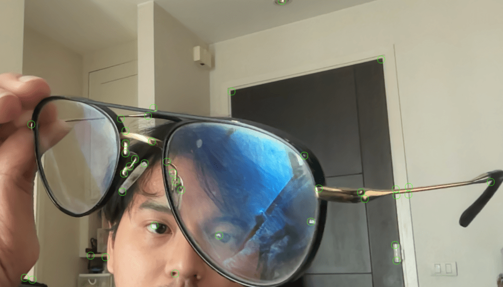
Image Feature and Alignment
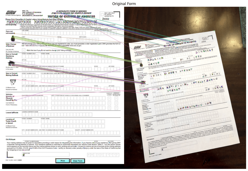
Image Alignment คือกระบวนการนำภาพที่มุมมองแตกต่างกันมาปรับให้ตรงกัน โดยใช้เทคนิคการจับคู่ฟีเจอร์ (Feature Matching) และการแปลง Homography
หลักการสำคัญที่ใช้ใน Image Alignment คือ Homography Transformation, ซึ่งเป็นการแปลงเชิงเรขาคณิตที่ใช้ในการ แมปจุดที่ตรงกันระหว่างสองภาพ โดยต้องใช้ จุดที่ตรงกันอย่างน้อย 4 จุด ในการคำนวณ Homography Matrix (H).
จากตัวอย่างในวีดิโอเขาจะทำการอ่านภาพสองมุม และทำการหา key features (ในที่นี้ใช้ ORB feature Oriented Fast and Rotated brief ซึ่งนิยมใช้ในการทำ image matching, object recognition, และ image alignment)
orb = cv2.ORB_create(MAX_NUM_FEATURES) ### MAX_NUM_FEATURES คือบอกว่าอยากได้กี่ point
keypoints1, descriptors1 = orb.detectAndCompute(im1_gray, None) ## หา keypoint และ compute descriptor
keypoints2, descriptors2 = orb.detectAndCompute(im2_gray, None)

# Display
im1_display = cv2.drawKeypoints(im1, keypoints1, outImage=np.array([]),
                                color=(255, 0, 0), flags=cv2.DRAW_MATCHES_FLAGS_DRAW_RICH_KEYPOINTS)

im2_display = cv2.drawKeypoints(im2, keypoints2, outImage=np.array([]),
                                color=(255, 0, 0), flags=cv2.DRAW_MATCHES_FLAGS_DRAW_RICH_KEYPOINTS)
| Parameters | Description |
| key-point | จุดเด่นในภาพ |
| descriptor | featured vector |

เมื่อเราได้ key features แล้วก็นำมาทำ features matching
# Match features.
matcher = cv2.DescriptorMatcher_create(cv2.DESCRIPTOR_MATCHER_BRUTEFORCE_HAMMING)

# Converting to list for sorting as tuples are immutable objects.
matches = list(matcher.match(descriptors1, descriptors2, None))

# Sort matches by score
matches.sort(key=lambda x: x.distance, reverse=False)

# Remove not so good matches
numGoodMatches = int(len(matches) * 0.1)
matches = matches[:numGoodMatches]
# Draw top matches
im_matches = cv2.drawMatches(im1, keypoints1, im2, keypoints2, matches, None)

plt.figure(figsize=[40, 10])
plt.imshow(im_matches);plt.axis("off");plt.title("Original Form")
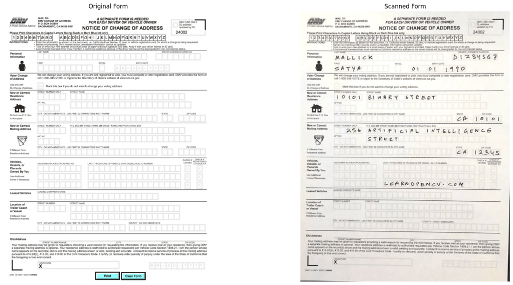
เมื่อได้จุดที่ match กันแล้วเราก็สามารถใช้การแปลงเชิงเรขาคณิตได้
# Extract location of good matches
points1 = np.zeros((len(matches), 2), dtype=np.float32)
points2 = np.zeros((len(matches), 2), dtype=np.float32)

for i, match in enumerate(matches):
    points1[i, :] = keypoints1[match.queryIdx].pt
    points2[i, :] = keypoints2[match.trainIdx].pt

# Find homography
h, mask = cv2.findHomography(points2, points1, cv2.RANSAC)
# Use homography to warp image
height, width, channels = im1.shape
im2_reg = cv2.warpPerspective(im2, h, (width, height))

# Display results
plt.figure(figsize=[20, 10])
plt.subplot(121);plt.imshow(im1);    plt.axis("off");plt.title("Original Form")
plt.subplot(122);plt.imshow(im2_reg);plt.axis("off");
plt.title("Scanned Form")
Panorama
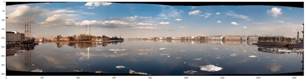
22. Create a panorama
Panorama คือการรวมภาพหลายๆ ภาพเข้าด้วยกันเพื่อสร้างภาพที่กว้างขึ้น ซึ่งเป็นเทคนิคที่ใช้ในงานด้าน Image Alignment และ Feature Matching
โดยปกติแล้วการทำภาพ Panoramas ต้องอาศัย 4 ขั้นตอนได้แก่
| Step | Process |
|---|---|
Detect Feature | ค้นหา Key Features ในแต่ละภาพ |
Match Keypoints | จับคู่ Key Features ระหว่างภาพ |
Estimate Homography | คำนวณ Homography Matrix เพื่อต่อภาพเข้าด้วยกัน |
Blend Images Smoothly | รวมภาพและทำให้ขอบภาพต่อกันอย่างแนบเนียน |
แต่ในตัวอย่างของ Course นี้จะใช้ built in function จาก Stitch Class ซึ่งเป็น automated high-level API ใช้งานง่าย สะดวกเหมาะกับการเรียนรู้พื้นฐาน แต่ ไม่เหมาะในกรณีที่ต้องการดัดแปลงภาพมากๆ หรือภาพ ไม่ได้ มีจุดต่อกันหลายจๆ จุด
# Stitch Images
stitcher = cv2.Stitcher_create()
status, result = stitcher.stitch(images)

if status == 0:
    plt.figure(figsize=[30,10])
    plt.imshow(result)
HDR
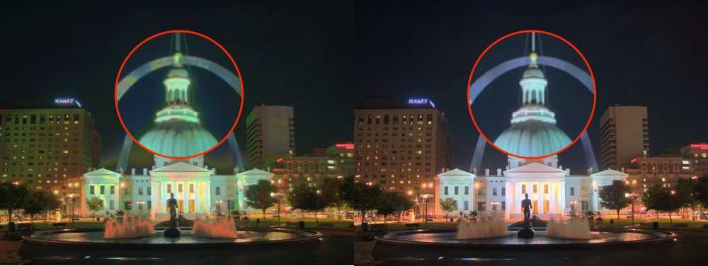
23. How to Make HDR Image using OpenCV
HDR (High Dynamic Range) เป็นเทคนิคที่ช่วยให้ภาพมี ช่วงสีและความสว่างที่กว้างขึ้น ทำให้สามารถเก็บรายละเอียดได้ทั้งในพื้นที่มืดและสว่างของภาพ
หลักการของ HDR คือการรวมภาพที่ถ่ายด้วย ค่า Exposure (EV) ต่างกัน เพื่อสร้างภาพที่มีรายละเอียดครบถ้วน
ในการสร้างภาพ HDR ในแล๊ปจะแบ่งออกเป็น 5 ขั้นตอน
1. อ่านชุดภาพที่มีค่า Exposure แตกต่างกัน
def readImagesAndTimes():
    # List of file names
    filenames = ["img_0.033.jpg", "img_0.25.jpg", "img_2.5.jpg", "img_15.jpg"]

    # List of exposure times
    times = np.array([1 / 30.0, 0.25, 2.5, 15.0], dtype=np.float32)

    # Read images
    images = []
    for filename in filenames:
        im = cv2.imread(filename)
        images.append(im)

    return images, times

2. Align ภาพให้ตรงกันด้วย createAlignMTB()
# Read images and exposure times
images, times = readImagesAndTimes()

# Align Images
alignMTB = cv2.createAlignMTB()
alignMTB.process(images, images)
- การจัดแนว (Alignment) ของภาพเป็นสิ่งสำคัญ เพราะหากภาพไม่ตรงกัน ภาพ HDR ที่ได้จะมี Ghosting
- เทคนิคที่ใช้คือ
Median Threshold Bitmap (MTB), ซึ่งทำงานโดยแปลงภาพเป็น Binary Mask และใช้ Bit-Shifting เพื่อจัดแนวภาพ
3. คำนวณ Camera Response Function (CRF)
# Find Camera Response Function (CRF)
calibrateDebevec = cv2.createCalibrateDebevec()
responseDebevec = calibrateDebevec.process(images, times)

# Plot CRF
x = np.arange(256, dtype=np.uint8)
y = np.squeeze(responseDebevec)

ax = plt.figure(figsize=(30, 10))
plt.title("Debevec Inverse Camera Response Function", fontsize=24)
plt.xlabel("Measured Pixel Value", fontsize=22)
plt.ylabel("Calibrated Intensity", fontsize=22)
plt.xlim([0, 260])
plt.grid()
plt.plot(x, y[:, 0], "b", x, y[:, 1], "g", x, y[:, 2], "r")
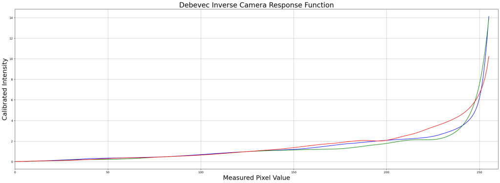
- ฟังก์ชัน
cv2.createCalibrateDebevec()คำนวณ Camera Response Function (CRF) เพื่อลดความผิดเพี้ยนของแสงในภาพ - ค่าที่ได้จาก CRF จะช่วยให้การรวมภาพ HDR แม่นยำขึ้น ลด Overexposure
4. สร้าง HDR Image
# Merge images into an HDR linear image
mergeDebevec = cv2.createMergeDebevec()
hdrDebevec = mergeDebevec.process(images, times, responseDebevec)
- ฟังก์ชัน
cv2.createMergeDebevec()รวมภาพทั้งหมดเป็น HDR โดยใช้ข้อมูลจาก CRF - ค่า
exposure_timesคือเวลาการเปิดรับแสงของแต่ละภาพ ซึ่งช่วยให้ระบบรู้ว่าภาพไหนสว่างกว่ากัน
5. ปรับโทนสีด้วย Tone Mapping
# Tonemap using Drago's method to obtain 24-bit color image
tonemapDrago = cv2.createTonemapDrago(1.0, 0.7)
ldrDrago = tonemapDrago.process(hdrDebevec)
ldrDrago = 3 * ldrDrago

# Saving image
cv2.imwrite("ldr-Drago.jpg", 255*ldrDrago)

# Plotting image
plt.figure(figsize=(20, 10));plt.imshow(np.clip(ldrDrago, 0, 1)[:,:,::-1]);plt.axis("off");
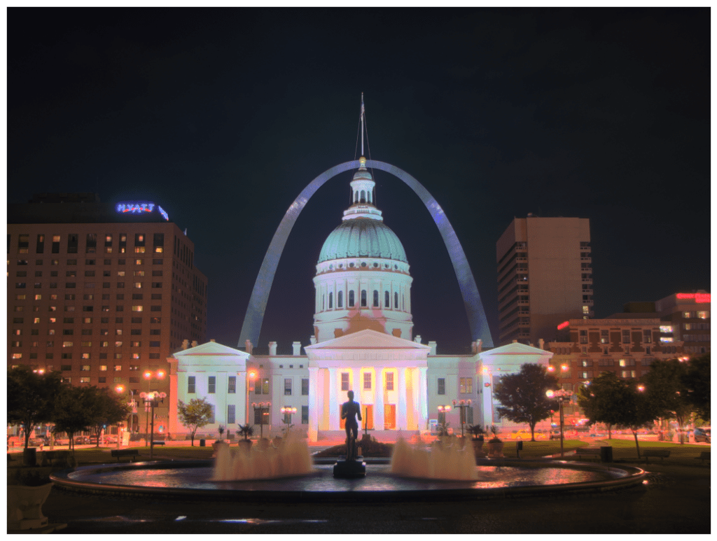
- การทำ Tone Mapping ช่วยปรับโทนสีให้สมดุลกับหน้าจอทั่วไป เพราะภาพ HDR มีค่าความสว่างสูงกว่าปกติ
- OpenCV มีหลาย Algorithm เช่น Drago, Reinhard, Mantiuk ซึ่งให้ผลลัพธ์ที่แตกต่างกัน
| Method | Description |
|---|---|
Drago | เหมาะกับภาพที่มี contrast สูง, ควบคุม Dynamic Range ได้ดี |
Reinhard | ปรับโทนสีให้สมดุลกับ การมองเห็นของมนุษย์ |
Mantiuk | เน้นการ เพิ่มรายละเอียดของภาพ |
Object Tracking
24. Real-time Tracking Object
Object Tracking คือกระบวนการติดตาม ตำแหน่งของวัตถุในวิดีโอ โดยใช้เฟรมแรกเป็นจุดเริ่มต้น และคำนวณตำแหน่งของวัตถุในเฟรมต่อๆ ไป
ใน OpenCV มีหลาย Algorithm ที่ใช้ในการติดตามวัตถุ ซึ่งแต่ละแบบมีจุดแข็งและจุดอ่อนที่แตกต่างกัน
| Algorithm | Description | Pros | Cons |
|---|---|---|---|
| BOOSTING | ใช้ AdaBoost Classifier | ใช้งานง่าย | ช้าและแม่นยำต่ำ |
| MIL | ใช้ Multiple Instance Learning | ทนต่อการเปลี่ยนแปลงของวัตถุ | อาจเกิด Drift ได้ |
| KCF | ใช้ Kernelized Correlation Filters | เร็วและแม่นยำกว่าทั่วไป | ไม่รองรับ Occlusion |
| CSRT | เน้นความแม่นยำสูง | แม่นยำมากกว่าทุกตัว | ช้ากว่า KCF |
| TLD | ใช้การเรียนรู้แบบ Self-learning | ฟื้นตัวจาก Occlusion ได้ดี | False Positives เยอะ |
| MEDIANFLOW | ใช้ Optical Flow คำนวณความแตกต่างของพิกเซล | แม่นยำสูงมาก | ใช้งานได้เฉพาะการเคลื่อนที่ Smooth |
| GOTURN | ใช้ Convolutional Neural Network (CNN) | ทนต่อการเปลี่ยนแปลงของวัตถุ | ต้องการ Pre-trained Model |
| MOSSE | ใช้ Minimum Output Sum of Squared Error | เร็วที่สุด เหมาะกับ real-time | ความแม่นยำต่ำ |
โค้ดด้านล่างจะเป็นการที่การอ่าน frame แรกและทำ กรอบสี่เหลี่ยมมล้อมบริเวรณที่วัตถุขยับ
เริ่มแรกก็จะเป็นฟังก์ชั่นที่เอาไว้วาดกรอบสำหรับติดตามวัตถุในวีดิโอและสำหรับเอาข้อความแสดง
video_input_file_name = "race_car.mp4"


def drawRectangle(frame, bbox):
p1 = (int(bbox[0]), int(bbox[1]))
p2 = (int(bbox[0] + bbox[2]), int(bbox[1] + bbox[3]))
cv2.rectangle(frame, p1, p2, (255, 0, 0), 2, 1)


def displayRectangle(frame, bbox):
plt.figure(figsize=(20, 10))
frameCopy = frame.copy()
drawRectangle(frameCopy, bbox)
frameCopy = cv2.cvtColor(frameCopy, cv2.COLOR_RGB2BGR)
plt.imshow(frameCopy)
plt.axis("off")


def drawText(frame, txt, location, color=(50, 170, 50)):
cv2.putText(frame, txt, location, cv2.FONT_HERSHEY_SIMPLEX, 1, color, 3)
# Set up tracker
tracker_types = [
"BOOSTING",
"MIL",
"KCF",
"CSRT",
"TLD",
"MEDIANFLOW",
"GOTURN",
"MOSSE",
]
เลือกประเภท Algorithm และอ่านเฟรมแรก
tracker_type = tracker_types[2]

if tracker_type == "BOOSTING":
tracker = cv2.legacy.TrackerBoosting.create()
elif tracker_type == "MIL":
tracker = cv2.legacy.TrackerMIL.create()
elif tracker_type == "KCF":
tracker = cv2.TrackerKCF.create()
elif tracker_type == "CSRT":
tracker = cv2.TrackerCSRT.create()
elif tracker_type == "TLD":
tracker = cv2.legacy.TrackerTLD.create()
elif tracker_type == "MEDIANFLOW":
tracker = cv2.legacy.TrackerMedianFlow.create()
elif tracker_type == "GOTURN":
tracker = cv2.TrackerGOTURN.create()
else:
tracker = cv2.legacy.TrackerMOSSE.create()
# Read video
video = cv2.VideoCapture(video_input_file_name)
ok, frame = video.read()
วน While Loop เพื่ออ่านแต่ละเฟรมและทำการบันทึกวีดิโอใหม่
# Exit if video not opened
if not video.isOpened():
print("Could not open video")
sys.exit()
else:
width = int(video.get(cv2.CAP_PROP_FRAME_WIDTH))
height = int(video.get(cv2.CAP_PROP_FRAME_HEIGHT))

video_output_file_name = "race_car-" + tracker_type + ".mp4"
video_out = cv2.VideoWriter(video_output_file_name, cv2.VideoWriter_fourcc(*"XVID"), 10, (width, height))

video_output_file_name
# Define a bounding box
bbox = (1300, 405, 160, 120)
# bbox = cv2.selectROI(frame, False)
# print(bbox)
displayRectangle(frame, bbox)
ok = tracker.init(frame, bbox)
while True:
ok, frame = video.read()

if not ok:
break

# Start timer
timer = cv2.getTickCount()

# Update tracker
ok, bbox = tracker.update(frame)

# Calculate Frames per second (FPS)
fps = cv2.getTickFrequency() / (cv2.getTickCount() - timer)

# Draw bounding box
if ok:
drawRectangle(frame, bbox)
else:
drawText(frame, "Tracking failure detected", (80, 140), (0, 0, 255))

# Display Info
drawText(frame, tracker_type + " Tracker", (80, 60))
drawText(frame, "FPS : " + str(int(fps)), (80, 100))

# Write frame to video
video_out.write(frame)

video.release()
video_out.release()
25. Real Time Face Detection
Face Detection
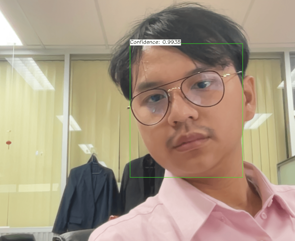
Face Detection เป็นเทคนิคที่ช่วยให้ระบบสามารถระบุใบหน้าของบุคคลในภาพหรือวีดิโอแบบเรียลไทม์ได้ โดยอาศัยฟังก์ชั่น cv2.dnn.readNetFromCaffe() ที่ใช้ในการดาวน์โหลดโมเดลที่เราฝึกไว้ล่วงหน้าแล้วได้
ในตัวอย่างนี้ เราจะใช้ Single Shot MultiBox Detector (SSD) ซึ่งเป็นโมเดลที่ถูกเทรนมาสำหรับ Face Detection และสามารถรันแบบเรียลไทม์ได้
ขั้นตอนการทำ
โหลด Pre-trained Model
เราควรใช้ cv2.dnn.blobFromImage() เพื่อแปลงภาพให้เหมาะสมกับโมเดล Deep Learning
import cv2

# โหลดโมเดลที่เทรนไว้ล่วงหน้า (SSD)
net = cv2.dnn.readNetFromCaffe("deploy.prototxt", "res10_300x300_ssd_iter_140000_fp16.caffemodel")
เปิดกล้องหรือโหลดวิดีโอ
cap = cv2.VideoCapture(0) # ใช้กล้องเว็บแคม
ประมวลผลเฟรมและตรวจจับใบหน้า
while cv2.waitKey(1) != 27:  # กด ESC เพื่อออก
    has_frame, frame = cap.read()
    if not has_frame:
        break

    frame = cv2.flip(frame, 1)  # แก้ปัญหา Mirror Effect ของกล้อง

    # สร้าง 4D blob สำหรับการทำ Neural Network Processing
    blob = cv2.dnn.blobFromImage(frame, 1.0, (300, 300), (104.0, 177.0, 123.0), swapRB=False, crop=False)

    # Run model เพื่อตรวจจับใบหน้า
    net.setInput(blob)
    detections = net.forward()
วาดกรอบรอบใบหน้าที่ตรวจพบ
ตั้งค่า Confidence ว่าถ้า เกิน 0.7 แปลว่าเป็นใบหน้าให้สร้างกรอบสีเขียว
 for i in range(detections.shape[2]):
        confidence = detections[0, 0, i, 2]

        if confidence > 0.7:  # กำหนด Threshold เพื่อกรองค่าที่ไม่แม่นยำออก
            # คำนวณตำแหน่งของกรอบใบหน้า
            h, w = frame.shape[:2]
            box = detections[0, 0, i, 3:7] * [w, h, w, h]
            x1, y1, x2, y2 = box.astype("int")

            # วาดกรอบสีเขียวรอบใบหน้า
            cv2.rectangle(frame, (x1, y1), (x2, y2), (0, 255, 0), 2)

            # แสดง Confidence Score
            label = f"Confidence: {confidence:.2f}"
            cv2.putText(frame, label, (x1, y1 - 10), cv2.FONT_HERSHEY_SIMPLEX, 0.5, (0, 255, 0), 2)
แสดงผลและปิดโปรแกรมเมื่อกด ESC
 cv2.imshow("Face Detection", frame)

cap.release()
cv2.destroyAllWindows()
26. What is behind. SSD Model
โมเดล SSD MobileNet ใช้เทคนิค Convolutional Neural Network (CNN) เพื่อตรวจจับใบหน้าในภาพ โดยใช้ Bounding Box และ Confidence Score
SSD MobileNet ถูกออกแบบมาให้มีขนาดเบา ใช้งานได้รวดเร็ว และเหมาะสำหรับอุปกรณ์ที่มีข้อจำกัดด้านพลังประมวลผล เช่น Mobile Devices หรือ Embedded Systems”
TF Object Detection
27. TF Object Detection
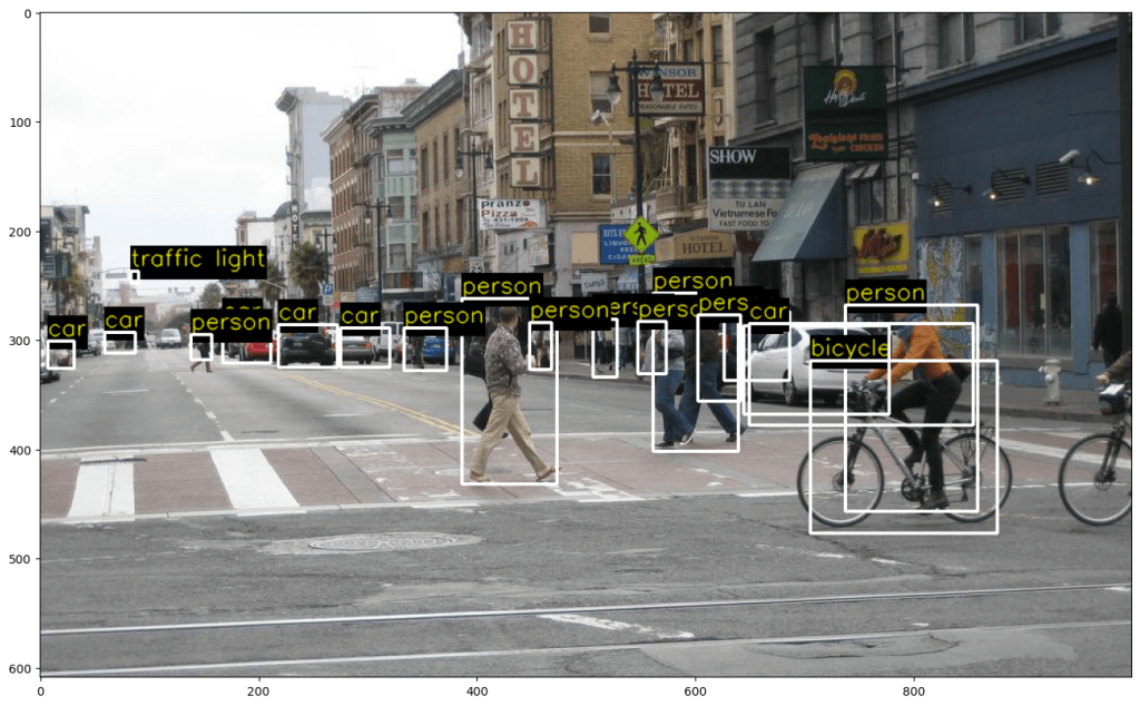
Object Detection คือกระบวนการระบุและจำแนกวัตถุภายในภาพหรือวิดีโอ ซึ่งเป็นพื้นฐานของ AI Vision เช่น Face Recognition, Autonomous Vehicles และ Security Systems
ใน Lab นี้ เราจะใช้ SSD MobileNet V2 ซึ่งเป็นโมเดลที่มีประสิทธิภาพสูงและเบาสำหรับการตรวจจับวัตถุแบบเรียลไทม์
ดาวน์โหลดและติดตั้งโมเดล
import os
import urllib.request
import tarfile

# ตรวจสอบว่ามีโฟลเดอร์ models หรือยัง
if not os.path.isdir("models"):
    os.mkdir("models")

# ตั้งค่าชื่อไฟล์โมเดล
model_url = "http://download.tensorflow.org/models/object_detection/ssd_mobilenet_v2_coco_2018_03_29.tar.gz"
model_path = "models/ssd_mobilenet_v2_coco_2018_03_29.tar.gz"

# ดาวน์โหลดโมเดลหากยังไม่มี
if not os.path.isfile(model_path):
    urllib.request.urlretrieve(model_url, model_path)

    # แตกไฟล์
    with tarfile.open(model_path, "r:gz") as tar:
        tar.extractall("models")

    # ลบไฟล์ tar.gz หลังจากแตกไฟล์เสร็จ
    os.remove(model_path)
SSD MobileNet V2 สามารถดาวน์โหลดจาก TensorFlow Model Zoo และใช้งานได้ทันที
โหลดโมเดลเข้าสู่ OpenCV
เราสามารถใช้ โมเดลจาก Tensorflow ด้วยการเรียก cv2.dnn.readNetFromTensorFlow()
modelFile  = os.path.join("models", "ssd_mobilenet_v2_coco_2018_03_29", "frozen_inference_graph.pb")
configFile = os.path.join("models", "ssd_mobilenet_v2_coco_2018_03_29.pbtxt")
# Read the Tensorflow network
net = cv2.dnn.readNetFromTensorflow(modelFile, configFile)
อ่านภาพและแปลงเป็นไฟล์ blob
# โหลดภาพตัวอย่าง
frame = cv2.imread("sample_image.jpg")

# แปลงภาพเป็น Blob
blob = cv2.dnn.blobFromImage(frame, 1.0, size=(300, 300), mean=(127.5, 127.5, 127.5), swapRB=True, crop=False)

# ส่งข้อมูลเข้าโมเดล
net.setInput(blob)
detections = net.forward()
ตรวจจับวัตถุและดึงข้อมูลพร้อมทั้งเขียนข้อความประกอบวัตถุนั้น
ตรวจจับวัตถุและกำหนดกรอบ Bounding Box เฉพาะวัตถุที่มีค่า Confidence สูงกว่า 25%
import numpy as np

rows, cols = frame.shape[:2]
threshold = 0.25  # Confidence threshold

for i in range(detections.shape[2]):
    # ดึงค่าความมั่นใจของการตรวจจับ
    confidence = detections[0, 0, i, 2]

    if confidence > threshold:
        classId = int(detections[0, 0, i, 1])
        x = int(detections[0, 0, i, 3] * cols)
        y = int(detections[0, 0, i, 4] * rows)
        w = int(detections[0, 0, i, 5] * cols - x)
        h = int(detections[0, 0, i, 6] * rows - y)

        # วาดกรอบและแสดงชื่อวัตถุ
        cv2.rectangle(frame, (x, y), (x + w, y + h), (0, 255, 0), 2)
        label = f"Class {classId} - {confidence:.2f}"
        cv2.putText(frame, label, (x, y - 10), cv2.FONT_HERSHEY_SIMPLEX, 0.5, (255, 255, 0), 1)
แสดงผลของภาพ
import matplotlib.pyplot as plt

plt.figure(figsize=(8, 6))
plt.imshow(cv2.cvtColor(frame, cv2.COLOR_BGR2RGB))
plt.axis("off")
plt.title("Object Detection Result")
plt.show()
Pose Estimation using OpenPose
28. Realtime Multi-Person 2D Pose Estimation using Part Affinity Field
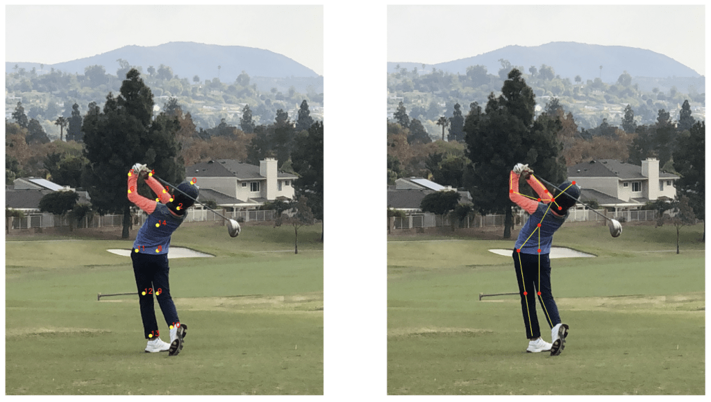
Pose Estimation คือการติดตาม จุดสำคัญของร่างกาย (Keypoints) ของบุคคลในภาพหรือวิดีโอแบบเรียลไทม์ ซึ่งสามารถนำไปใช้ในงาน กีฬา, การเคลื่อนไหวของมนุษย์ (Human Motion Analysis), หรือแม้แต่ Virtual Reality (VR)
โดยในแล๊ปนี้เราจะใช้ OpenPose Deep Learning Model ที่สามารถตรวจจับ Key-points ได้หลายคน ( Multi-Person) โดยใช้ Part Affinity Fields (PAFs)
โหลด Pre-trained Model
ขั้นแรกเราต้องโหลดโมเดลที่ถูกเทรนมาแล้วกับข้อมูลขนาดใหญ่เพื่อนำมาจับท่าทางของคน
import cv2

# โหลดไฟล์โมเดลจาก OpenPose
protoFile = "pose_deploy_linevec_faster_4_stages.prototxt"
weightsFile = "pose_iter_160000.caffemodel"

# โหลดโมเดลเข้าสู่ OpenCV
net = cv2.dnn.readNetFromCaffe(protoFile, weightsFile)
อ่านภาพและแปลงเป็น Blob
# อ่านภาพจากกล้องหรือไฟล์
frame = cv2.imread("person.jpg")

# แปลงภาพเป็น Blob
blob = cv2.dnn.blobFromImage(frame, 1.0 / 255, (368, 368), (0, 0, 0), swapRB=False, crop=False)

# ส่งข้อมูลเข้าโมเดล
net.setInput(blob)
output = net.forward()
อย่าลืมแปลงภาพเป็น blob สำหรับการทำ Deep Learning
ดึง Keypoints ที่ตรวจพบ
กรอง keypoint ที่อยู่ต่ำกว่าค่า threshold ออกด้วย cv2.minMaxLoc()
import numpy as np

nPoints = 15  # จำนวน Keypoints ในโมเดล OpenPose
h, w = frame.shape[:2]

# คำนวณ Scale Factor
scaleX = w / output.shape[3]
scaleY = h / output.shape[2]

# เก็บตำแหน่ง Keypoints
points = []

# ค่าความมั่นใจขั้นต่ำ
threshold = 0.1

for i in range(nPoints):
    probMap = output[0, i, :, :]
    minVal, prob, minLoc, point = cv2.minMaxLoc(probMap)

    x = int(point[0] * scaleX)
    y = int(point[1] * scaleY)

    if prob > threshold:
        points.append((x, y))
    else:
        points.append(None)
วาด Key-points และ Skeleton
ค้ดนี้ใช้ cv2.circle() เพื่อวาด Keypoints และ cv2.line() เพื่อเชื่อมต่อ key-points เป็น Skeleton
POSE_PAIRS = [
    [0, 1], [1, 2], [2, 3], [3, 4], [1, 5], [5, 6], [6, 7],
    [1, 14], [14, 8], [8, 9], [9, 10], [14, 11], [11, 12], [12, 13]
]

# วาด Keypoints
for i, p in enumerate(points):
    if p:
        cv2.circle(frame, p, 5, (0, 255, 0), -1)
        cv2.putText(frame, str(i), p, cv2.FONT_HERSHEY_SIMPLEX, 0.5, (255, 0, 0), 1)

# วาด Skeleton
for pair in POSE_PAIRS:
    partA, partB = pair

    if points[partA] and points[partB]:
        cv2.line(frame, points[partA], points[partB], (255, 0, 0), 2)
แสดงผลลัพธ์ ด้วย MatplotLib
import matplotlib.pyplot as plt

plt.figure(figsize=(8, 6))
plt.imshow(cv2.cvtColor(frame, cv2.COLOR_BGR2RGB))
plt.axis("off")
plt.title("Pose Estimation Result")
plt.show()
จบกันไปแล้วนะครับกับ สิ่งที่ผมได้รู้จากคอร์สฟรีที่ OpenCV University เกี่ยวกับ OpenCV โดยในหัวข้อนี้จะเน้นไปที่การอธิบาย โค้ดเป็นหลักอาจะไม่ได้ลงลึกในด้านวิชาคณิตสาสตร์ ขอผมไปศึกษาก่อนแล้วจะกลับมาเขียนในหัวข้อถัดไป ละเพื่อนๆคิดว่าจากตัวอย่างทั้งหมด อันไหนดูน่าจะประยุกต์ใช้ได้ง่ายสุดครับลองมาแชร์กันได้ครับ

Leave a comment